Chainrisk VaR Methodology

Value at Risk (VaR) widely adopted by both traditional and DeFi institutions to gauge potential losses within portfolios under varying market conditions. In DeFi, VaR’s relevance has grown as protocols seek robust methodologies to manage bad debt and counter extreme market volatilities. 

This blog explores the core principles of VaR, its calculation methods—including historical simulation, variance-covariance, and Monte Carlo simulation—and its critical applications within financial risk management.

Introduction to VaR

Value at Risk (VaR) is a statistical measure used in finance to quantify the level of risk within a portfolio or investment over a specific time frame. VaR, inspired from the statistical concept of variance 𝛔²  is used to capture the variance that can be present in the observed potential loss under different market conditions. 

One of the use cases of VaR is to estimate the maximum potential loss with a given confidence level (usually 95% or 99%) under various market conditions. For example, a one-day VaR at the 95% confidence level of $1 million means there is a 95% probability that the institutions (or Portfolio in traditional finance) will not lose more than $1 million in one day. 

VaR can be found widely in any literature of traditional financial markets. However, it is also being used extensively to understand the potential bad debt (loss) that can be incurred by Decentralized Financial (DeFi) institutions as well, like protocols and others.

Value-at-Risk (VaR) : Statistical Estimate for Financial Risk Management

In financial risk management, alpha (ɑ) is the probability of experiencing extreme losses and is directly tied to the calculation of Value at Risk (VaR). VaR is estimated at a specific confidence level, which is defined as 1-ɑ. For instance, if ɑ=0.05, this corresponds to a 95% confidence level, meaning there is a 5% chance that losses will exceed the VaR threshold within a given time period.

By selecting different values of alpha, risk managers can adjust the strictness of VaR estimates, with lower alpha values (higher confidence levels) indicating more conservative risk assessments. 

‍

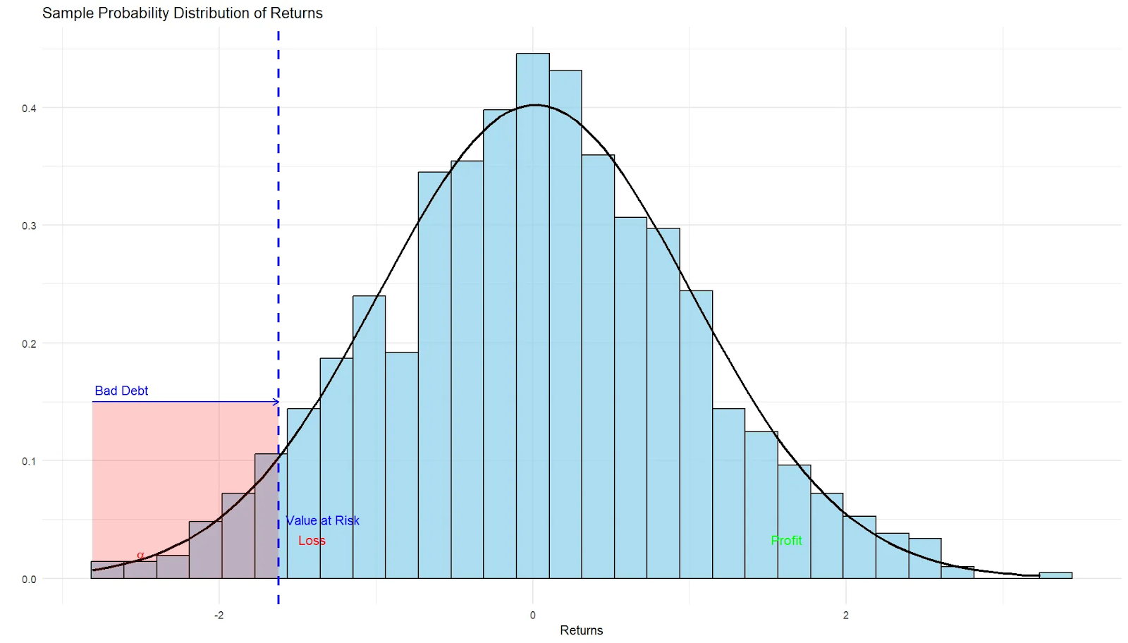
This relationship between alpha and VaR allows institutions to set risk limits based on their tolerance for extreme loss scenarios. The VaR depicted in the graph corresponds to the 95th percentile of the distribution, and any loss below that point is an extreme bad debt (loss).

Types of VaR Calculation Methods

VaR, a statistical estimate of the spread of the DeFi institutes loss can be computed in numerous ways. Some of which are just touched upon in this section.

• Historical Simulation: Uses actual historical returns data to estimate potential future losses, assuming past trends may resemble future behavior.
• Variance-Covariance (Parametric) Method: Assumes normal distribution of returns and uses the mean and standard deviation of returns to estimate VaR. It’s efficient but less accurate for returns having non-linear instruments (e.g., options).
• Monte Carlo Simulation: Generates numerous random scenarios to simulate potential losses. This method is flexible but computationally intensive, providing a more thorough risk assessment.

Simulation-Based Calculation for Estimating Value at Risk (VaR)

Initial Simulation

Start with a set of simulations (say for sake of illustration, $2000$) using an initial set of model parameters, s. These parameters have been decided upon using the historical price data. 

After these simulations, calculate the 95th percentile (say X_i) of the resulting losses. This represents the loss level that has only a 5% chance of being exceeded, giving an initial bad-debt estimate.

Convergence Check

To confirm the reliability of the 95th percentile estimate, conduct an additional set of simulations using the same model parameters, s as done earlier. Now, we recalculate the 95th percentile (say X_i+1) bad debt based on the new appended observed bad-debt values. 

The two observed 95th percentile values are compared. If the difference X_i+1-X_i is within a specified tolerance level 𝝐 ,i.e., X_i+1-X_i  ⩽𝝐, then X_i+1 is considered as the VaR. 

If not, additional simulations are done until the difference is within the tolerance limit.

Applications of VaR in Risk Management

Value at Risk (VaR) plays a vital role in risk management by providing institutions with a clear measure of potential losses, allowing them to navigate market uncertainties with confidence. This section explores how VaR is applied in practical settings to maintain financial stability, support balanced growth, and prepare for extreme market conditions.

Establishing Risk Limits

Financial institutions set specific risk limits for portfolios or trading activities based on VaR calculations, ensuring that investments remain within the organization’s risk tolerance and support capital preservation. This helps prevent excessive risk-taking by aligning daily operations with long-term financial stability goals.

Augmenting Stress Testing

Although VaR focuses on normal market conditions, pairing it with stress testing allows institutions to assess how portfolios might perform during extreme, atypical events. This combination provides a more complete risk profile, helping firms prepare for and withstand unexpected shocks.

Supporting Strategic Decision-Making

Firms use VaR insights to proactively adjust portfolio allocations, avoiding overexposure to riskier assets. This helps align investment strategies with both market conditions and the organization’s risk appetite, enhancing resilience and promoting balanced growth.

Extreme VaR

To simulate usual market conditions, and understand the market dynamics in a more general way, we use the 95th percentile values. Also we can use a more rigorous condition of taking the 99th percentile value in place of the 95th value, which can help us to check for the extreme market conditions and check for the extreme market scenarios.

Conclusion

Value at Risk (VaR) is a powerful tool that helps financial institutions measure and manage potential losses, keeping risk within acceptable limits. Whether in traditional finance or DeFi, VaR’s various calculation methods—like historical simulation and Monte Carlo simulation—offer flexible ways to understand and prepare for potential downturns. As markets face constant shifts, VaR remains essential for helping organizations stay steady through uncertainty, ensuring that they’re equipped to handle unexpected challenges while keeping their financial strategies on track.

‍